 Some time ago when we looked at modelling the simple example of Hezekiah’s tunnel (EPANET Network Components – Database tables and rows, Part 1 (#18)), we discussed the options for creating our data tables including some ways to use a class hierarchy. EPANET has nodes (junctions, reservoirs and tanks) and links (pipes, pumps and valves) which connect two nodes.
Nodes have a few shared characteristics, such as location, and these can be added to a general node class from which all the different node types inherit. Links have a node at each end, so each link must point to two different nodes: one as its start node and the other as its end node.
This is simple modelling, but the more complex question is how we will handle the sub-classing. In a recent series of newsletters, we looked at the performance differences between the different sub-classing options available in Django, and now we need to apply this knowledge in a practical way.
The three sub-classing options we considered need to be customised slightly to fit with our need for three types of nodes. The options are:
Option 1 – A single nodes table
A single table called “NODESA” contains the junction-, reservoir- and tank-specific attributes, as well as the common node attributes. Unused attributes for junctions, reservoirs or tanks are set to NULL or similar values. In our performance tests, selection was the area where this modelling option took 50% longer than either of the other options.
Option 2 – A table for each type of node
Three tables – a ‘JUNCTIONB’, ‘RESERVOIRB’ and ‘TANKB’ table – are defined, each of which contains both shared node attributes and some attributes specific to the type of node. Our performance testing showed deletion to be the area where this modelling option performed badly, taking more than twice as long as either of the other options.
Option 3 – Shared base table
The “node” information is stored in a ‘NODEC’ table, while the information about the junction aspect of junctions is included in a ‘JUNCTIONC’ table, the reservoir-specific aspects of reservoirs are stored in a table called ‘RESERVOIRC’. and the tank-specific aspects of tanks are stored in a table called ‘TANKC’. Our performance testing showed that the creation of large numbers of objects with this modelling option performed badly since the bulk_create() function cannot be used with multi-table inheritance.
So let’s work through the list of requirements from our last newsletter and see which sub-classing option would be most likely to give us the best performance. I have numbered the items in the list this time so that we can refer to them.
We said that our modelling must facilitate speedy:
- loading of the data for a distribution network from a file.
- deletion of all data relating to a network modelling project.
- adding, editing and deleting of individual objects as part of the design process.
- searching for existing objects in the database.
- analysis of a distribution network stored in the database.
These operations map fairly easily to various underlying database operations as shown in the table below:
| Number | Summary | Database operation |
|---|---|---|
| 1 | Project import | Bulk insert |
| 2 | Project deletion | Bulk deletion |
| 3 | Project editing | Limited add/edit/delete |
| 4 | Search and view | Bulk or limited selection |
| 5 | Analysis | Bulk selection, possibly bulk update |
Using the results of performance analysis for the different methods of sub-classing, we can see the sort of performance we might expect for each of these activities, and we plan to do this in the next post.


Leave A Comment